Sometimes you just want to get a bunch of data typed into an easy to use piece of software and know you can get that data back out summarized however you might need it. That data might be cattle records, your expenses for the year, or some other information. Excel is made to summarize data and starting with Excel 2007 it is actually easy enough for the occasional user.
Example: Summarize Your Checkbook
Let’s say you want to summarize last year’s checkbook in time for this year’s tax extension. This is a really simple example, but of course it’s far better to do your books using QuickBooks or some other accounting software. Remember, though, that this technique works for any kind of data where you have a lot of similar items you’d like to summarize. That makes it a good technique to learn.
In our example, you only wrote the following 8 checks for the year:
| Check # | Date | Vendor | Amount | Memo |
| 1121 | 1/31/2010 | Ranch and Farm | 1,259.12 | $1000 supplies, $200 repairs, $59.12 personal stuff |
| 1122 | 2/28/2010 | Reynolds Warehouse | 659.00 | $75 supplies, the rest groceries |
| 1123 | 4/29/2010 | Dawson County Vet Clinic | 3,899.00 | $752.00 supplies, $3147 vet |
| 1124 | 7/31/2010 | Ranch and Farm | 7,988.00 | $1250 supplies, $234 personal, rest repairs |
| 1125 | 8/31/2010 | Farmers Union | 15,243.00 | $10,000 fertilizer, $5243 fuel |
| 1126 | 11/15/2010 | Reynolds Warehouse | 1,247.50 | $240.50 supplies, $1007 groceries |
| 1127 | 11/15/2010 | Farmers Union | 6,210.00 | fuel |
Entering Your Checks
Enter each piece of information from your checks on ONE row. That’s the key – you have to make this simple for Excel. That first check happens to have three pieces of information – supplies, repairs, personal – so it needs three rows. That check number will be listed on that three consecutive rows. The last check is only one piece of information because the entire amount goes to Fuel Expense. Most checks will be like the last check.
Enter your deposits on a separate tab. It’s just easier that way.
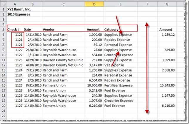
Here’s an example of how I’d build the spreadsheet. There are a couple of important things to note about this example:
- The Headings are bold and the rest of the text isn’t. The headings sit exactly on the top of the first row of data. Those two things are important. Excel needs the headings to be formatted differently than the rest of the data.
- There are NO blank rows or blank columns in the actual data. That is critical. An occasional blank cell doesn’t hurt anything but we don’t have any in this data.
- There is an important blank row between column E and Column G because I don’t want to use Column G in my data – I want to summarize on the amounts in Column D not on the whole check amounts from Column G. Why have G at all? You don’t have to. I used it to double check myself that my item amounts in D all totaled the same as the check totals in G did. Since we won’t use it in the summaries, it has to have that blank column between it and the data we want to summarize. Ditto the totals at the bottom (which aren’t visible in the picture.
- The same category name is always identical. “Supplies Expense” is always exactly that and never “Supplies Exp.” Or “Supp.” Or any of the other abbreviations that a human will instantly recognize as the same and Excel will not. Excel needs the same things to be identical. Just make use of the auto-complete function in Excel and as soon as it guesses the right thing, hit the tab button. Faster and more accurate. You may also want to summarize by Vendor and so it’s good to use the same name there too.
Summarizing Using a PivotTable
Entering data is the hard part. Now for the FUN!
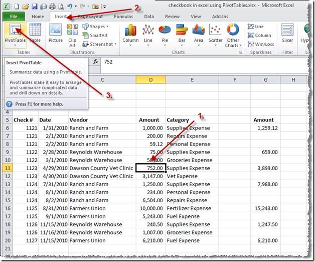
Insert a PivotTable on a new sheet.
- Click in the middle of the data you want to summarize.
- Click the Insert Ribbon
- Click the first button on the Insert Ribbon – it says PivotTable.
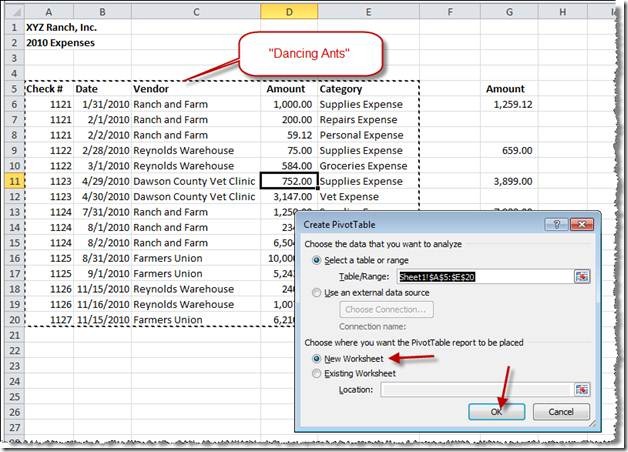
Make sure it is defaulting to the correct information for the dialog box. Choose to select a table or range. The range should be the data you want to summarize without the data that you don’t. If you look at the spreadsheet, you’ll see the “dancing ants” selection surrounding exactly and only the data you want to summarize. You also want to put this in a new spreadsheet because it’s way easier to manage that way. Usually, the defaults will be correct and you can just check them and click OK.
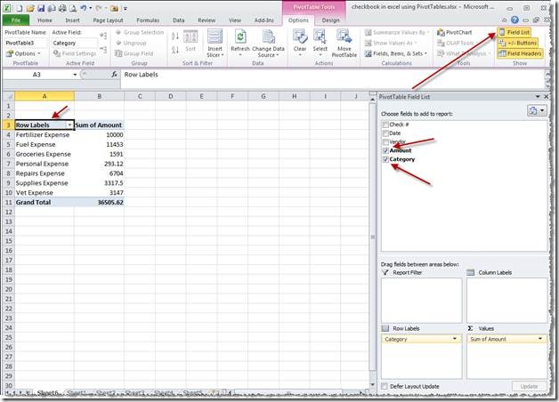
Excel will make a new tab in your workbook and it will look a little useless for a minute. Don’t worry. Over on the right side of your screen you can see a panel called the PivotTable Field List. The top section says, “Choose fields to add to your report.” You click on the checkboxes in from of Amount and Category to choose them. They are, really, all you need right now.
If the fields list panel isn’t showing, just click on the Field List toggle button on the PivotTable ribbon. Also, it will disappear if you don’t have a cell inside the PivotTable as the active cell. Just click back into the middle of the summarized data to bring it back.
Magically (well, it seems like it!) Excel will take all that data from your original spreadsheet and total it by expense category. How cool is that?
Of course this feature is extremely powerful and huge amounts of data can be analyzed in complex ways using PivotTables. That flexibility makes playing with PivotTables a great idea. Once you get the hang of them, you will find other uses for this powerful feature.
Troubleshooting
Of course these directions assume everything went perfectly. That doesn’t always happen with computers.
Some things to check if you don’t have the magic work. By the way, the best way to correct a problem with a PivotTable is usually to just do it over – faster and cleaner and more likely to work.
DO NOT type anything into a column that you need to summarize mathematically. For example, it’s tempting to type the word “VOID” in the amount for a voided check. But that is text and you need to only have numbers in the Amount column, expect for the heading itself. You’ll confuse Excel if you put text in there and it won’t be able to do the match you need. So put a zero in the amount column for voided checks and save the work VOID for comments or even the vendor name.
Good luck! And remember, we are always interested in your feedback about improving a tutorial.


